| Issue |
Natl Sci Open
Volume 5, Number 1, 2026
Special Topic: Intelligent Materials and Devices
|
|
|---|---|---|
| Article Number | 20250048 | |
| Number of page(s) | 16 | |
| Section | Materials Science | |
| DOI | https://doi.org/10.1360/nso/20250048 | |
| Published online | 08 December 2025 | |
RESEARCH ARTICLE
Real-time cross-domain monitoring of multi-UAV-multi-USV systems via efficient block sparse Bayesian learning
1
School of Artificial Intelligence and Automation, Institute of Artificial Intelligence, Engineering Research Center of Autonomous Intelligent Unmanned Systems (Ministry of Education), Huazhong University of Science and Technology, Wuhan 430074, China
2
Guangdong HUST Industrial Technology Research Institute, Huazhong University of Science and Technology, Dongguan 523808, China
3
School of Artificial Intelligence, Optics and ElectroNics (iOPEN), Northwestern Polytechnical University, Xi’an 710072, China
* Corresponding author (email: This email address is being protected from spambots. You need JavaScript enabled to view it.
)
Received:
14
September
2025
Revised:
27
November
2025
Accepted:
5
December
2025
Abstract
Despite the tremendous progress in coordinating multi-unmanned surface vehicle (USV) fleets, persistent monitoring remains a dilemma because USVs cannot share data with external monitors. Practical deployments further impose real-time constraints and limited onboard calculation capability, necessitating low-complexity algorithms. This study proposes a multi-UAV fleet-based monitoring scheme. Therein, UAVs are assigned to pairwise USV-UAV matching to observe relative positionreal time. An efficient block sparse Bayesian learning algorithm (EBSBL) is then developed to identify the coordinated dynamics of USVs, with theoretically guaranteed feasibility. In addition, the unscented Kalman filter (UKF) is employed to facilitate multi-UAV coordinated monitoring with real-time prediction and USV trajectory estimation. The effectiveness and superiority of the proposed method are demonstrated by both numerical simulations and real-lake based multi-UAV-multi-USV platform experiments.
Key words: cross-domain monitoring / unmanned surface vehicles (USVs) / unmanned aerial vehicles (UAVs) / sparse Bayesian learning (SBL)
© The Author(s) 2025. Published by Science Press and EDP Sciences.
 This is an Open Access article distributed under the terms of the Creative Commons Attribution License (https://creativecommons.org/licenses/by/4.0), which permits unrestricted use, distribution, and reproduction in any medium, provided the original work is properly cited.
INTRODUCTION
Recent developments in machine learning algorithms and sensor technologies have facilitated the integration of autonomous systems in real-world marine applications, such as environmental monitoring [1-3], disaster response [4, 5], and industrial automation [6, 7]. Unmanned surface vehicles (USVs) have emerged as indispensable tools, enabling a wide variety of missions [8-10]. Despite the tremendous progress in multi-USV fleet coordination, real-time monitoring remains a dilemma when USVs are noncooperative and do not share data with external monitors. Furthermore, practical deployments impose constraints on real-time efficiency and limited onboard calculation capability, necessitating low-complexity algorithms.
A global positioning system (GPS)-based tracking control system for wheeled mobile robots is introduced in such unmanned systems, which compensates for skidding and slipping effects using real time kinematic (RTK)-GPS, ensuring navigational trajectory tracking [11]. In Ref. [12], a vision-based target detection and localization system is developed, utilizing a cooperative swarm composed of UAVs and unmanned ground vehicles (UGVs), where UAVs employ an optical flow for motion detection and UGVs make individual detection. In Ref. [13], a vehicle monitoring system is developed by integrating an Arduino microcontroller with global system for mobile communications (GSM) and GPS modules. A framework for adaptive learning navigation with nested guidance layers is introduced in Ref. [14] for UAVs, enabling horizontal monitoring and vertical descent in confined landing zones using solely relative position feedback. However, these schemes depend on motion information directly provided by the non-cooperative monitored targets. To address this issue, a target-tracking control system for underactuated autonomous surface vehicles (ASVs) is proposed in Ref. [15], which relies solely on line-of-sight range and angle measurements. Moreover, this system integrates an extended state observer and a single hidden layer neural network to estimate both target dynamics and external disturbances. A monocular camera-based method was proposed in Ref. [16], leveraging optical flow for target localization, and integrating it with an extended Kalman filter (EKF) to estimate motion dynamics. Furthermore, Ref. [17] establishes a hierarchical coarse-to-fine deep reinforcement learning framework for UAV tracking, where a coarse stage initializes the bounding box, and a fine stage refines it to handle aspect-ratio, scale, and occlusion changes. However, these approaches rely on ideal models, which exhibit high computational complexity. To analyze multi-source data, Ref. [18] develops a UAV-based tracking-and-recognition system integrating consensus-based tracking, neural-network detection, and gimbal stabilization, where real-time tracking is achieved via multimodal fusion together with moving-background compensation. A tracking system for USVs is tailored, utilizing an EKF and a visibility-aware control strategy to enhance target detection, positioning accuracy, and trajectory prediction [19]. Additionally, Ref. [20] introduces a target detection method with the assistance of a single shot multibox detector, a support vector machine classifier, and a tracking algorithm. Despite these advancements, few existing studies address the scenario of multi-target coordinated monitoring.
To this end, we design a cooperative method for multi-USV systems. The UAVs are assigned according to USV-UAV pairwise matching to observe relative positions online. An efficient block sparse Bayesian learning algorithm (EBSBL) with low computational complexity is proposed to identify the coordinated dynamics of the multi-USV fleet, leveraging the advantages of sparse Bayesian learning (SBL) over traditional  methods for sparse, high-quality signal recovery, and incorporating structural information for improved performance [21, 22]. Additionally, the unscented Kalman filter (UKF) is employed to facilitate real-time prediction, USV trajectory estimation, and UAV monitoring coordination. In summary, the contributions of this work are two-fold.
(1) Propose a real-time cross-domain monitoring method not requiring motion information provided by the multi-USV fleet.
(2) Propose an EBSBL with theoretically guaranteed feasibility.
The remainder of this paper is organized as follows. Section PRELIMINARIES AND PROBLEM FORMULATION introduces the problem addressed by the paper with necessary preliminaries. Section METHOD develops the monitoring scheme, which includes UAVs assignment, coordinated dynamics learning, and cross-domain coordinated tracking modules. Experiments are conducted on a self-established cross-domain platform in Section NUMERICAL AND EXPERIMENTAL RESULTS to demonstrate both the effectiveness and superiority of the proposed monitoring method. Finally, the conclusion is drawn in Section CONCLUSIONS.
PRELIMINARIES AND PROBLEM FORMULATION
Consider a multi-UAV-multi-USV scenario where  USVs are monitored by
  UAVs, as shown in Figure 1. Denote the positions of the
  -th USV
  ,
,  , where
  and
and  represent the position along the
  - and
- and  -axes of the
  -th USV, respectively. Denote the positions of the
  -th UAV
  ,
,  , where
  and
and  represent the positions along the
  - and
- and  -axes of the
  -th UAV, respectively, and
  represents the fixed altitude. Assume that the dynamics of USVs
  is governed by the velocity function
  , which is widely applied in cooperative control of USVs as follows[23-25]:
 (1)The dynamics of USVs are represented by the following kinematic model [26]:
 (2)where
  represents the rotation matrix, and
  ,
,  , and
, and  are the orientation angle, forward velocity, and transverse velocity, respectively. The dynamics of UAVs is modeled as follows:
 (3)where
  and
and  denote the velocity and control input of the
  -th UAV, respectively.
 |
Figure 1 Diagram of the algorithm for UAVs monitoring (or tracking) USVs with EBSBL, consisting of three stages. Stage 1: Assign UAVs to USVs using auction algorithm and make observations. Stage 2: Identify USV dynamics using efficient block sparse Bayesian learning. Stage 3: Monitor USVs in coordination using identified results and UKF by UAVs. |
Note that the USVs do not share their position and velocity information with the UAVs, which can only be observed by the UAVs. More precisely, during the observation period, each UAV can observe any USV, rather than being restricted to a fixed pairwise monitoring scheme. Define the relative position of the  -th USV observed by the
  -th UAV at time
  as
as 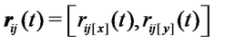 , where
  and
and  represent the relative positions along the
  - and
- and  -axes, respectively. Denote
  as the time when the observation is not available. The problem addressed by this paper is motivated as below.
Problem 1: Monitor the USVs by identifying the dynamics of USVs  and predicting their positions
  based on the relative observed data
  and the positions
  of UAVs, i.e.,
  .
.
METHOD
UAVs assignment for tracking USVs
To enable trajectory observation and tracking of USVs, each USV is assigned to a unique UAV at each observation time  , which inspires to the following pairwise matching optimization problem:
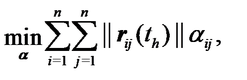 (4a)
(4a) (4b)where
  is a binary variable equal to
  if the
  -th USV is assigned to the
  -th UAV, and otherwise. The objective function (4a) seeks to minimize the total observation distance, given that the quality of UAV-collected data deteriorates with increasing distance. Furthermore, when the UAV is closer to the target, it can more rapidly follow the trajectory of USV. To solve problem (4), the auction algorithm [27] is employed, which iteratively alternates between a bidding phase and an assignment phase. In the bidding phase, for each unassigned
  -th USV, i.e.,
  , the reward function is defined as
 (5)where
  denotes the current price of
  -UAV, initialized as
  . The optimal and suboptimal UAVs for the
  -th USV are determined as
 (6)Accordingly, the
  -th USV submits a bid to
  -th UAV given by
 (7)where
  is a small positive constant. In the assignment phase, each UAV is allocated to the USV offering the highest bid, i.e.,
 (8)the price of the
  -th UAV is then updated as
  . If the
  -th UAV was previously assigned to another USV
  , the earlier assignment is canceled, i.e.,
  , and the new allocation is established with
  .
.
Remark 1. The assignment problem in Eq. (4) imposes the one-to-one matching constraints in Eq. (4a), which ensures that each USV is assigned to exactly one UAV at each observation time  . When the numbers of UAVs and USVs are equal, these constraints define a matching between the two sets. Combined with the auction-based solution procedure, which iteratively assigns all remaining unassigned USVs, the proposed method guarantees that all USVs are observed at each observation time [27].
Define the total observation time as  , the observation number of the
  -th USV by the
  -th UAV as
  ,
,  . Building on the allocation matrix
  obtained from Eq. (4), the estimated position of the
  -th USV by its assigned the
  -th UAV at time
  is described as
 (9)Thereby, the trajectory of the
  -th USV can be expressed as
  , and the velocity
  is approximated by using the Euler method.
Coordinated dynamics with efficient block sparse Bayesian learning
An EBSBL is proposed to identify the coordinated dynamics of USVs. To approximate the unknown velocity function  , we build up the vector of candidate functions
  composed of nonlinear candidate functions, where
  denotes the number of functions. Define
  as follows:
 (10)where
  denotes the current observation number. Define the set of time observations associated with the
  -th UAV of the
  -th USV as
  , the vector of weights to be identified as
  ,
,  ,
,  ,
,  , one has
 (11)where
  denotes the current observation number of the
  -th USV by the
  -th UAV.
Since the proposed method independently identifies the coordinated dynamics of each USV in both  - and
- and  - directions, the subscripts
  ,
,  , and
, and  are omitted for conciseness. For the
  - and
- and  -axes dynamics of the
  -th USV, define data vector
  and dictionary matrix
  stacked from all
  and
and  , respectively, as follows:
 (12)and the elements of
  are defined as follows:
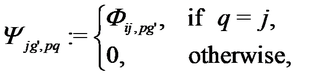 (13)where
  and
and  denote the elements in the
  -th row and
  -th column of
  and the
  -th row and
  -th column of
  , respectively,
  . Define
  stacked from all
  as follows:
 (14)where
  denotes the
  -th element of
  . As a result, one has
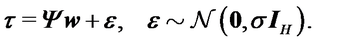 (15)
(15)
Block prior is introduced as follows: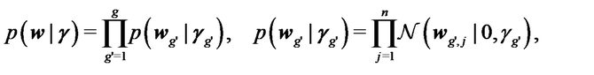 (16)where
  denotes the
  -th element of
  ,
,  ,
,  . Define an auxiliary variable
  , and the likelihood function
  can be written as [28]
 (17)where
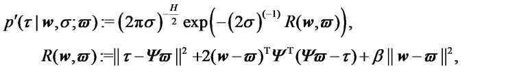 (18)
(18) ,
,  is a small positive constant, and
  denotes eigenvalues. We use the strict lower bound function
  of the likelihood function
  to compute the posterior distribution of
  , as follows:
 (19)where
  is the estimated fixed vector, and the posterior covariance
  and mean
  of
of  are given by
 (20)The purpose is to estimate the unknown parameters
  ,
,  , and
, and  using the evidence maximization method [28], the optimal values of
  and
and  are obtained by maximizing the marginalized probability density function
  as follows:
 (21)where the last inequality is obtained by swapping the order of integration and maximization [28]. As a result,
 (22)with
 (23)Taking
  of Eq. (22), we obtain the following objective function to be minimized:
 (24)with
  . From Eq. (20), one has
  As a result,
 (25)Note that
  , one has
 (26)Therefore, the joint objective function is obtained as follows:
 (27)with
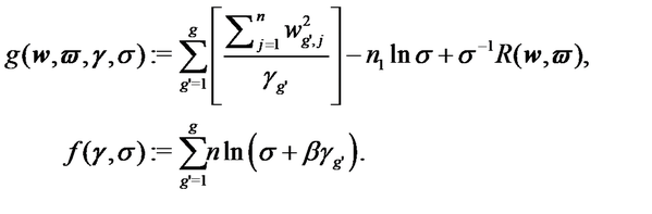 (28)Note that
  is convex with respect to
  , and
, and  is concave with respect to
  . Hence,
  is a convex-concave procedure problem [29], which can be solved as follows:
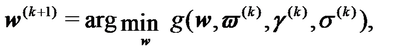 (29a)
(29a)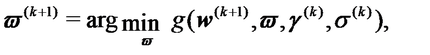 (29b)
(29b) (29c)
(29c) (29d)Since the objective functions in Eqs. (29a)–(29c) are convex, setting the gradient to zero yields:
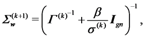 (30a)
(30a)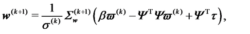 (30b)
(30b) (30c)
(30c) (30d)
(30d) (30e)
(30e) (30f)The final
  is obtained by averaging over each block
  in
in  as follows:
 (31)
(31)
Note that Eq. (30a) only involves the inversion of a diagonal matrix, which has an operation of  . Consider the matrix multiplication
  in Eq. (30b), the proposed EBSBL has a computational complexity of
  . In contrast, for conventional block sparse Bayesian learning algorithm [30], each iteration requires computing the inverse of a non-diagonal matrix, resulting in
  computational complexity. As a result, EBSBL reduces the computational complexity from
  to
to  .
.
Then, the coordinated dynamics  of the
  -th USV can be identified as follows:
 (32)
(32)
Theorem 1. The sequence  generated using EBSBL is non-increasing and locally convergent. Moreover,
  is bounded.
Proof. Define the surrogate function  as follows:
 (33)As
  is an affine function and
  is convex, one has
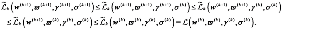 (34)The concavity of
  leads to
 (35)Therefore, the sequence
  is non-increasing. Since
  ,
,  , and
, and  , the cost function
  is lower bounded. By the monotone convergence theorem [31], the nonincreasing sequence
  is locally convergent. Hence, the sequence
  is bounded, which completes the proof.
Cross-domain coordinated tracking
The UKF [32] is employed in this system to predict the position of USVs by handling the nonlinear dynamics. Unlike EKF, the UKF does not require linearization, making it more suitable for complex systems. UKF generates sigma points around the current state estimate and propagates them through the nonlinear model, providing more accurate state and covariance estimates. While direct trajectory estimation based on USV dynamics does not account for uncertainties such as sensor inaccuracies and environmental disturbances, UKF integrates the dynamics model with measurements in a probabilistic framework. It iteratively updates the trajectory estimate using the relative position data observed by UAVs, correcting the estimate at each time step based on the new measurement and the predicted state from the previous step.
Let  and
and  denote the posterior estimated position and the estimated position from the previous step of
  -th USV, respectively, where
  represents the time step. The predicted position
  of the
  -th USV at the current time
  is obtained from the previous state estimate
  and the system’s dynamic model
  . The UKF predicts the position at the current time step as follows:
 (36)UKF generates a set of sigma points
  to approximate the probability distribution of the system state, which are derived from the current state estimate
  and the associated covariance matrix, describing the uncertainty in the current state estimate. The sigma points
  are generated and propagated through the system model as follows:
 (37)where
  is a scaling parameter, and
  the column vectors of the square root of the covariance matrix
  . The predicted states are yielded as follows:
 (38)where
  denotes the sigma points propagated through
  over
over  , and
, and  are the weights associated with each sigma point. The predicted covariance is given by
 (39)where
  are the covariance weights associated with each sigma point,
  represents the external noise covariance. The new sigma points
  are generated using the updated
  and
and  . The measurement update step involves generating predicted measurements
  from the predicted sigma points, using the measurement function
 (40)The measurement covariance S and cross-covariance C are given by
 (41)where
  is the measurement noise covariance. The Kalman gain in UKF is computed as
  . The current state estimate
  and updated covariance
  are updated as follows:
 (42)
(42)
The controller for the  -th UAV to monitor the
  -th USV is designed as follows [33]:
 (43)where
 (44)
(44) and
and  are the proportional and derivative gains, respectively. To avoid collisions among UAVs, a potential field-based controller is utilized for UAVs. The repulsive force
  exerted on the
  -th UAV by
  -th UAV is defined as follows [34]:
 (45)where
  is the repulsive force coefficient. According to Ref. [35], the controller
  of the
  -th UAV is
 (46)where
  is a positive gain parameter. As a result, the control input of UAVs is as follows:
 (47)
(47)
The complete monitoring procedures are summarized in Algorithm 1 with the associated diagram shown in Figure 1.
Multi-UAV-multi-USV monitoring with EBSBL (MUMU-EBSBL)
NUMERICAL AND EXPERIMENTAL RESULTS
Setups
In this section, we demonstrate the effectiveness and superiority of the proposed MUMU-EBSBL by both numerical simulation and real-lake experiments. For comparison, we construct three variants by replacing the EBSBL module with mainstream system identification methods, i.e., block SBL (BSBL) [30], vanilla SBL (VSBL) [36], and LASSO [37], yielding MUMU-BSBL, MUMU-VSBL, and MUMU-LASSO, respectively. The MUMU framework and all the other settings are kept identical across variants. Circular formation [25] and line formation [8] are selected for the coordinated dynamics of USVs.
In numerical simulations, we consider four UAVs monitoring four USVs. In real-lake experiments, we introduce a self-developed cross-domain platform, including three HUSTER-12c USVs and three M-200 UAVs. As shown in Figure 2(a) and (b), the HUSTER-12c USV has a length of 1.2 m and a width of 0.42 m. It is equipped with two CA-6152A GPS antennas, an STM32F407 control module, and a TP-Link TLBS520 Wi-Fi module. Each M-200 UAV measures 0.65 m in both length and width, and is fitted with a DJI Matrice 200 Series GPS module, a Manifold 2 control module, and the same TP-Link TLBS520 Wi-Fi module. Figure 2(c) shows the coordination workflow of the cross-domain platform. UAVs track the positions of USVs through observation and establish communication using a WiFi 5G network, allowing them to generate the required guidance signals for navigation. The base station receives and logs all states, including positions, tracking errors, etc., transmitted over the WiFi 5G network. To quantify the performance of the algorithms, the error metric is defined as  .
.
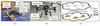 |
Figure 2 Architecture of the real-lake experimental platform. (a) HUSTER-12c USV, (b) M-200 UAV, and the detailed components. (c) Operation procedure of the cross-domain monitoring system, which consists of three HUSTER-12c USVs, three M-200 UAVs, and a WiFi 5G (TP-link TLBS520) wireless communication station. USVs and UAVs have independent communication networks, with USVs not sharing information with UAVs. |
Numerical simulation results
Figure 3 shows the tracking errors evolution of numerical simulations with circular formation. Figure 3(a) presents the tracking error results for four USVs under the proposed MUMU-EBSBL algorithm. The errors decrease steadily over time, demonstrating the effectiveness of MUMU-EBSBL. Figure 3(b) compares performance of the four algorithms at 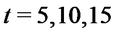 s. It is observed that all the algorithms exhibit decreasing tracking errors, whereas the proposed MUMU-EBSBL always achieves the best performance with a considerable margin. For
  s, the error of MUMU-EBSBL is below
  m, indicating satisfactory performance. For
  s, the average error of MUMU-EBSBL is reduced by
  ,
,  , and
, and  relative to MUMU-BSBL, MUMU-VSBL, and MUMU-LASSO, respectively.
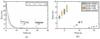 |
Figure 3 The tracking errors evolution of numerical simulations with circular formation. (a) The tracking errors of four USVs under MUMU-EBSBL. (b) The errors comparison among MUMU-EBSBL, MUMU-BSBL, MUMU-VSBL, and MUMU-LASSO at |

Figure 4 shows the tracking errors evolution of numerical simulations with line formation, where Figure 4(a) presents the results under MUMU-EBSBL, demonstrating that UAVs successfully track USVs. Figure 4(b) compares performance of the four algorithms at  s. It is observed that MUMU-EBSBL always achieves the best performance among all the four algorithms. For
  s, the average error of MUMU-EBSBL is more accurate than all other algorithms with the reduction of
  ,
,  , and
, and  , compared with MUMU-BSBL, MUMU-VSBL, and MUMU-LASSO, respectively. The effectiveness and superiority of the proposed MUMU-EBSBL are thus verified.
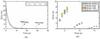 |
Figure 4 The tracking errors evolution of numerical simulations with line formation. (a) The tracking errors of four USVs under MUMU-EBSBL. (b) The errors comparison among MUMU-EBSBL, MUMU-BSBL, MUMU-VSBL, and MUMU-LASSO at |

Real-lake experimental results
Figure 5 shows the experimental snapshots and tracking errors evolution of real-lake experiments with circular formation. Figure 5(c) presents the tracking errors evolution for three USVs under MUMU-EBSBL. It is observed that tracking errors gradually decrease. Figure 5(d) shows tracking errors for the four algorithms at  s. The results indicate that MUMU-EBSBL consistently outperforms the other algorithms. At
  s, the error of MUMU-EBSBL is reduced by
  ,
,  , and
, and  relative to MUMU-BSBL, MUMU-VSBL, and MUMU-LASSO, respectively. Equivalently, for
  s, the error of MUMU-EBSBL is
  ,
,  , and
, and  of that of MUMU-BSBL, MUMU-VSBL, and MUMU-LASSO, respectively.
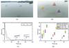 |
Figure 5 The experimental snapshots and the tracking errors evolution of real-lake experiments with circular formation, where blue circles denote USVs, yellow circles denote UAVs, and red circle denotes trajectory. (a) Initial scene with USVs at their starting positions. (b) UAVs performing real-time tracking and monitoring of the motion of USVs. (c) The tracking errors of three USVs under MUMU-EBSBL. (d) The tracking errors comparison among MUMU-EBSBL, MUMU-BSBL, MUMU-VSBL, and MUMU-LASSO at |
Figure 6 illustrates the experimental snapshots and tracking errors evolution of real-lake experiments with line formation, where Figure 6(c) presents the results under the proposed MUMU-EBSBL. It is observed that tracking errors gradually decrease, demonstrating the effectiveness of the proposed MUMU-EBSBL. Figure 6(d) shows the comparison of tracking errors among MUMU-EBSBL, MUMU-BSBL, MUMU-VSBL, and MUMU-LASSO. The results indicate that MUMU-EBSBL yields the best tracking performance among all four algorithms. For  s, the error of MUMU-EBSBL is
  ,
,  , and
, and  of that of MUMU-BSBL, MUMU-VSBL, and MUMU-LASSO, respectively. In addition, the error of MUMU-EBSBL for
  s is reduced by
  ,
,  , and
, and  relative to MUMU-BSBL, MUMU-VSBL, and MUMU-LASSO, respectively. Both the effectiveness and superiority of MUMU-EBSBL are thus demonstrated.
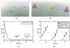 |
Figure 6 The experimental snapshots and the tracking errors evolution of real-lake experiments with line formation, where blue circles denote USVs, yellow circles denote UAVs, and red line denotes trajectory. (a) Initial scene with USVs at their starting positions. (b) UAVs performing real-time tracking and monitoring of the motion of USVs. (c) The tracking errors of three USVs under MUMU-EBSBL. (d) The tracking errors comparison among MUMU-EBSBL, MUMU-BSBL, MUMU-VSBL, and MUMU-LASSO at |

CONCLUSION
This paper proposes a real-time cross-domain monitoring strategy, i.e., MUMU-EBSBL, for multi-UAV-multi-USV fleet. UAVs are pairwise matched to USVs for real-time relative positioning, USV coordinated dynamics are identified via a convergence-guaranteed EBSBL, and a UKF enables monitoring with real-time prediction and trajectory estimation. The virtue of the proposed MUMU-EBSBL lies in the elimination of the requirement on motion information of the multi-USV fleet while maintaining low computational cost. Both effectiveness and superiority are demonstrated through numerical simulations and real-lake multi-USV experiments. Future research will focus on noncooperative UAVs monitoring of USVs that actively evade sensing.
Data availability
The original data are available from corresponding authors upon reasonable request.
Funding
This work was supported by the National Natural Science Foundation of China (62225306, U2141235), the National Key R&D Program of China (2022ZD0119601), and the HUST Taihu Lake Innovation Fund for Future Technology (2024B5).
Author contributions
Y.Z. and H.T.Z. developed the real-time cross-domain monitoring algorithms. Y.Z. and J.H. developed the codes and experiments. Y.Z., J.H., and B.X. carried out the experiments. Y.Z., H.T.Z., J.H., B.X, and J.D. participated in designing and discussing the study and writing the paper.
Conflict of interest
The authors declare no conflict of interest.
Supplementary information
Supplementary file provided by the authors. Access Supplementary Material
The supporting information is available online at https://doi.org/10.1360/nso/20250048. The supporting materials are published as submitted, without typesetting or editing. The responsibility for scientific accuracy and content remains entirely with the authors.
References
- Guan X. Network system capacity: Towards integrating sensing, communication and control. Nat Sci Open 2024; 3: 20230036.[Article] [Google Scholar]
- Susca S, Bullo F, Martinez S. Monitoring environmental boundaries with a robotic sensor network. IEEE Trans Contr Syst Technol 2008; 16: 288–296.[Article] [Google Scholar]
- Wang G, Liu X, Xiao Y, et al. Extinction chains reveal intermediate phases between the safety and collapse in mutualistic ecosystems. Engineering 2024; 43: 89–98.[Article] [Google Scholar]
- Wang G, Liu X, Chen G, et al. Indirect effects among biodiversity loss of mutualistic ecosystems. Nat Sci Open 2022; 1: 20220002.[Article] [Google Scholar]
- Savkin AV, Huang H. Range-based reactive deployment of autonomous drones for optimal coverage in disaster areas. IEEE Trans Syst Man Cybern Syst 2021; 51: 4606–4610.[Article] [Google Scholar]
- Gonzalez AGC, Alves MVS, Viana GS, et al. Supervisory control-based navigation architecture: A new framework for autonomous robots in industry 4.0 environments. IEEE Trans Ind Inf 2018; 14: 1732–1743.[Article] [Google Scholar]
- Czimmermann T, Chiurazzi M, Milazzo M, et al. An autonomous robotic platform for manipulation and inspection of metallic surfaces in industry 4.0. IEEE Trans Automat Sci Eng 2022; 19: 1691–1706.[Article] [Google Scholar]
- Liu B, Zhang HT, Meng H, et al. Scanning-chain formation control for multiple unmanned surface vessels to pass through water channels. IEEE Trans Cybern 2022; 52: 1850–1861.[Article] [Google Scholar]
- Tang C, Zhang HT, Wang J. Flexible formation tracking control of multiple unmanned surface vessels for navigating through narrow channels with unknown curvatures. IEEE Trans Ind Electron 2023; 70: 2927–2938.[Article] [Google Scholar]
- Cao H, Hu BB, Mo X, et al. The immense impact of reverse edges on large hierarchical networks. Engineering 2024; 36: 240–249.[Article] [Google Scholar]
- Low Chang Boon, Wang Danwei. GPS-based tracking control for a car-like wheeled mobile robot with skidding and slipping. IEEE ASME Trans Mechatron 2008; 13: 480–484.[Article] [Google Scholar]
- Minaeian S, Liu J, Son YJ. Vision-based target detection and localization via a team of cooperative UAV and UGVs. IEEE Trans Syst Man Cybern Syst 2016; 46: 1005–1016.[Article] [Google Scholar]
- Sun N, Zhao J, Shi Q, et al. Moving target tracking by unmanned aerial vehicle: A survey and taxonomy. IEEE Trans Ind Inf 2024; 20: 7056–7068.[Article] [Google Scholar]
- Zhang HT, Hu BB, Xu Z, et al. Visual navigation and landing control of an unmanned aerial vehicle on a moving autonomous surface vehicle via adaptive learning. IEEE Trans Neural Netw Learn Syst 2021; 32: 5345–5355.[Article] [Google Scholar]
- Liu L, Wang D, Peng Z, et al. Bounded neural network control for target tracking of underactuated autonomous surface vehicles in the presence of uncertain target dynamics. IEEE Trans Neural Netw Learn Syst 2019; 30: 1241–1249.[Article] [Google Scholar]
- Nabavi-Chashmi SY, Asadi D, Ahmadi K. Image-based UAV position and velocity estimation using a monocular camera. Control Eng Pract 2023; 134: 105460.[Article] [Google Scholar]
- Zhang W, Song K, Rong X, et al. Coarse-to-fine UAV target tracking with deep reinforcement learning. IEEE Trans Automat Sci Eng 2019; 16: 1522–1530.[Article] [Google Scholar]
- Wang S, Jiang F, Zhang B, et al. Development of UAV-based target tracking and recognition systems. IEEE Trans Intell Transp Syst 2020; 21: 3409–3422.[Article] [Google Scholar]
- Huang T, Xue Y, Xue Z, et al. USV-tracker: A novel USV tracking system for surface investigation with limited resources. Ocean Eng 2024; 312: 119196.[Article] [Google Scholar]
- Liu Y, Wang Q, Hu H, et al. A novel real-time moving target tracking and path planning system for a quadrotor UAV in unknown unstructured outdoor scenes. IEEE Trans Syst Man Cybern Syst 2019; 49: 2362–2372.[Article] [Google Scholar]
- Wipf DP, Rao BD, Nagarajan S. Latent variable Bayesian models for promoting sparsity. IEEE Trans Inform Theor 2011; 57: 6236–6255.[Article] [Google Scholar]
- Baraniuk RG, Cevher V, Duarte MF, et al. Model-based compressive sensing. IEEE Trans Inform Theor 2010; 56: 1982–2001.[Article] [Google Scholar]
- Xu Z, He S, Zhou W, et al. Path following control with sideslip reduction for underactuated unmanned surface vehicles. IEEE Trans Ind Electron 2024; 71: 11039–11047.[Article] [Google Scholar]
- Kou L, Chen Z, Xiang J. Cooperative fencing control of multiple vehicles for a moving target with an unknown velocity. IEEE Trans Automat Contr 2022; 67: 1008–1015.[Article] [Google Scholar]
- Liu B, Chen Z, Zhang HT, et al. Collective dynamics and control for multiple unmanned surface vessels. IEEE Trans Contr Syst Technol 2020; 28: 2540–2547.[Article] [Google Scholar]
- Hu BB, Zhang HT, Shi Y. Cooperative label-free moving target fencing for second-order multi-agent systems with rigid formation. Automatica 2023; 148: 110788.[Article] [Google Scholar]
- Bertsekas DP. The auction algorithm: A distributed relaxation method for the assignment problem. Ann Oper Res 1988; 14: 105–123.[Article] [Google Scholar]
- Zhou W, Zhang HT, Wang J. An efficient sparse Bayesian learning algorithm based on Gaussian-scale mixtures. IEEE Trans Neural Netw Learn Syst 2022; 33: 3065–3078.[Article] [Google Scholar]
- Yuille AL, Rangarajan A. The concave-convex procedure (CCCP). In: Proceedings of the 15th International Conference on Neural Information Processing Systems: Natural and Synthetic. Vancouver, 2002. 1033–1040 [Google Scholar]
- Zhang Z, Rao BD. Extension of SBL algorithms for the recovery of block sparse signals with intra-block correlation. IEEE Trans Signal Process 2013; 61: 2009–2015.[Article] [Google Scholar]
- Bartle RG, Sherbert DR. Introduction to Real Analysis. New York: Wiley, 2000 [Google Scholar]
- Shen H, Wen G, Lv Y, et al. USV parameter estimation: Adaptive unscented kalman filter-based approach. IEEE Trans Ind Inf 2023; 19: 7751–7761.[Article] [Google Scholar]
- Thomas J, Welde J, Loianno G, et al. Autonomous flight for detection, localization, and tracking of moving targets with a small quadrotor. IEEE Robot Autom Lett 2017; 2: 1762–1769.[Article] [Google Scholar]
- Wu Z, Hu G, Feng L, et al. Collision avoidance for mobile robots based on artificial potential field and obstacle envelope modelling. Assem Autom 2016; 36: 318–332.[Article] [Google Scholar]
- Abeywickrama HV, Jayawickrama BA, He Y, et al. Potential field based inter-UAV collision avoidance using virtual target relocation. In: Proceedings of the 2018 IEEE 87th Vehicular Technology Conference. Porto, 2018. 1–5 [Google Scholar]
- Wipf DP, Rao BD. Sparse Bayesian learning for basis selection. IEEE Trans Signal Process 2004; 52: 2153–2164.[Article] [Google Scholar]
- Tibshirani R. Regression shrinkage and selection via the lasso. J R Stat Soc Ser B-Stat Meth 1996; 58: 267–288.[Article] [Google Scholar]
All Tables
All Figures
|
Figure 1 Diagram of the algorithm for UAVs monitoring (or tracking) USVs with EBSBL, consisting of three stages. Stage 1: Assign UAVs to USVs using auction algorithm and make observations. Stage 2: Identify USV dynamics using efficient block sparse Bayesian learning. Stage 3: Monitor USVs in coordination using identified results and UKF by UAVs. |
| In the text | |
|
Figure 2 Architecture of the real-lake experimental platform. (a) HUSTER-12c USV, (b) M-200 UAV, and the detailed components. (c) Operation procedure of the cross-domain monitoring system, which consists of three HUSTER-12c USVs, three M-200 UAVs, and a WiFi 5G (TP-link TLBS520) wireless communication station. USVs and UAVs have independent communication networks, with USVs not sharing information with UAVs. |
| In the text | |
|
Figure 3 The tracking errors evolution of numerical simulations with circular formation. (a) The tracking errors of four USVs under MUMU-EBSBL. (b) The errors comparison among MUMU-EBSBL, MUMU-BSBL, MUMU-VSBL, and MUMU-LASSO at |
| In the text | |
|
Figure 4 The tracking errors evolution of numerical simulations with line formation. (a) The tracking errors of four USVs under MUMU-EBSBL. (b) The errors comparison among MUMU-EBSBL, MUMU-BSBL, MUMU-VSBL, and MUMU-LASSO at |
| In the text | |
|
Figure 5 The experimental snapshots and the tracking errors evolution of real-lake experiments with circular formation, where blue circles denote USVs, yellow circles denote UAVs, and red circle denotes trajectory. (a) Initial scene with USVs at their starting positions. (b) UAVs performing real-time tracking and monitoring of the motion of USVs. (c) The tracking errors of three USVs under MUMU-EBSBL. (d) The tracking errors comparison among MUMU-EBSBL, MUMU-BSBL, MUMU-VSBL, and MUMU-LASSO at |
| In the text | |
|
Figure 6 The experimental snapshots and the tracking errors evolution of real-lake experiments with line formation, where blue circles denote USVs, yellow circles denote UAVs, and red line denotes trajectory. (a) Initial scene with USVs at their starting positions. (b) UAVs performing real-time tracking and monitoring of the motion of USVs. (c) The tracking errors of three USVs under MUMU-EBSBL. (d) The tracking errors comparison among MUMU-EBSBL, MUMU-BSBL, MUMU-VSBL, and MUMU-LASSO at |
| In the text | |
Current usage metrics show cumulative count of Article Views (full-text article views including HTML views, PDF and ePub downloads, according to the available data) and Abstracts Views on Vision4Press platform.
Data correspond to usage on the plateform after 2015. The current usage metrics is available 48-96 hours after online publication and is updated daily on week days.
Initial download of the metrics may take a while.